Features
The code is very flexible and can easily be extended to include new setups
and algorithms. Some of the implemented features are presented below:
Particle Push
Particle push is the procedure that updates both the position and
velocity of each particle based on the electric and magnetic fields at
the location of the particle. Position and velocity are leap-frogged
over each other, that is they are defined at half a timestep offset from
each other. This makes the scheme second order accurate in time.
Boris Push
Usually the code uses the original Boris push in the relativistic
version as defined in Boris, 1970. (The paper is annoyingly hard to
find. It was titled
Relativistic plasma simulation - optimization of
a hybrid code and was published in the Proceedings of the Fourth
Conference on Numerical Simulation Plasmas.)
Vay Modification
For simulations where particles reach more than mildly relativistic
velocities the code also implements the modifications to the Boris push
that were proposed by
Vay, 2008.
Staggered Grid
Unlike many Eulerian codes that have all components of the fields that
are stored in the grid located at the center of each grid cell, it is
common in particle-in-cell codes to have different field components at
different locations. This is especially useful for the commonly used
electromagnetic plasma model, where the update of the field quantities
in time requires the use of the curl of the dual field. The most widely
used arrangement, which is also used in ACRONYM, is the so called Yee
lattice, as proposed by
Yee, 1966. In
principle the locations of the electric and magnetic fields can be
interchanged without losing the advantageous properties, however we have
decided on the layout shown below, as it makes the implementation of
perfect electric conductors easier.
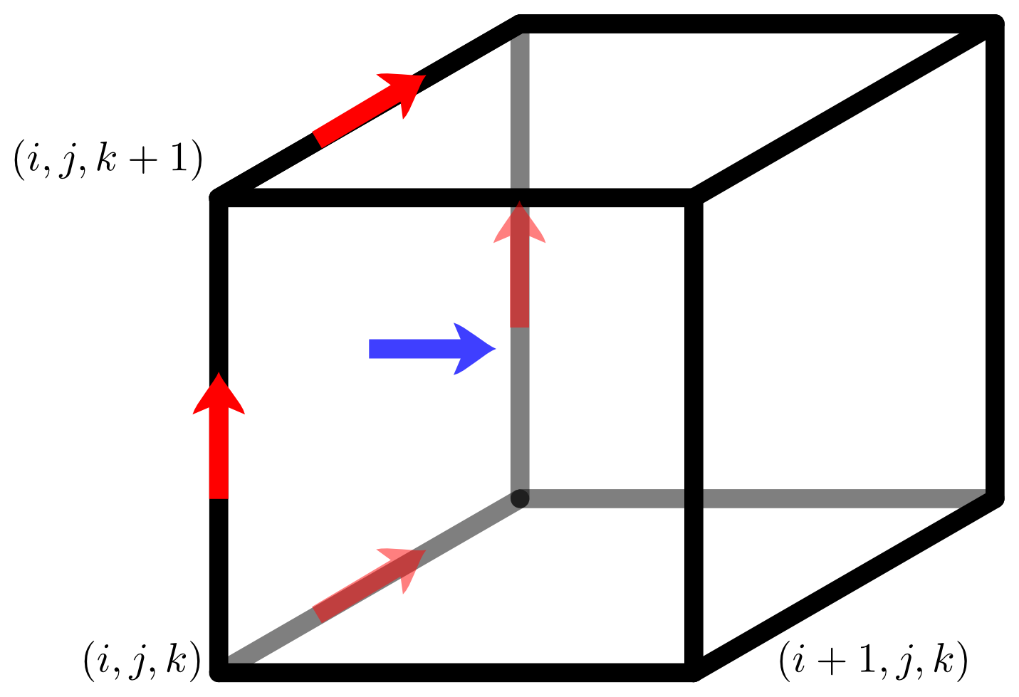
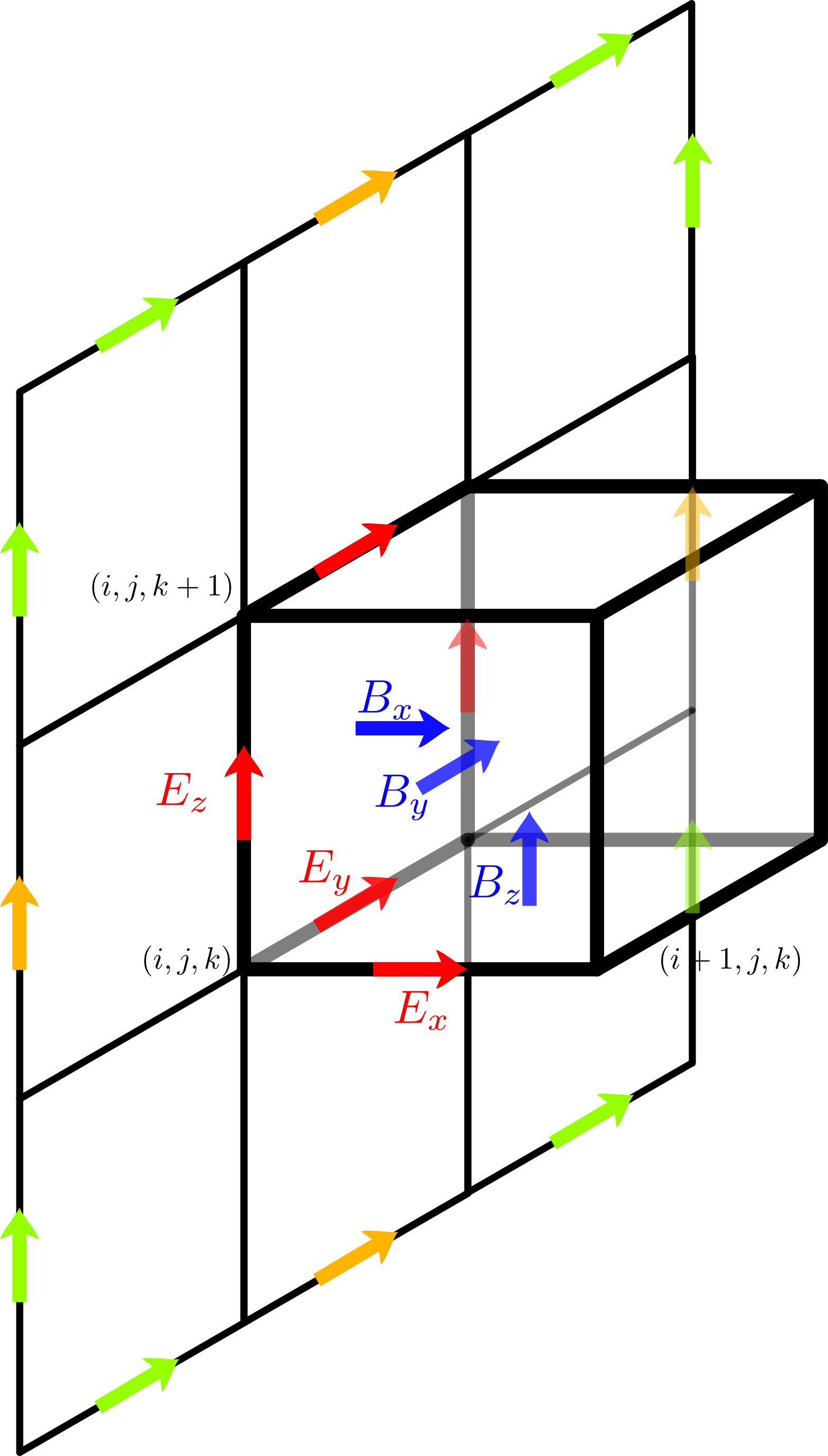
Electric Field
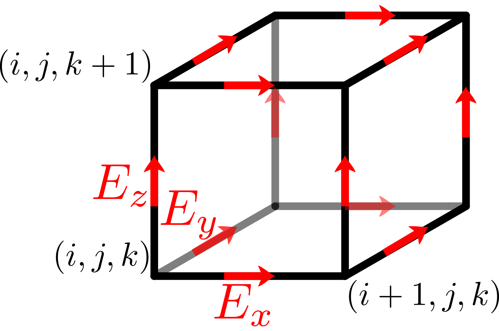
The electric field components are located at grid edges, displaced to
the center of the edge that is aligned with the direction of the field
component. That is the x component E_x of the electric field is
displaced by half a grid spacing dx along the edge e_x.
For a perfectly electrically conducting wall at x=0, this arrangement
locates the y and z component exactly at the surface of the conductor,
where they are trivially forced to zero.
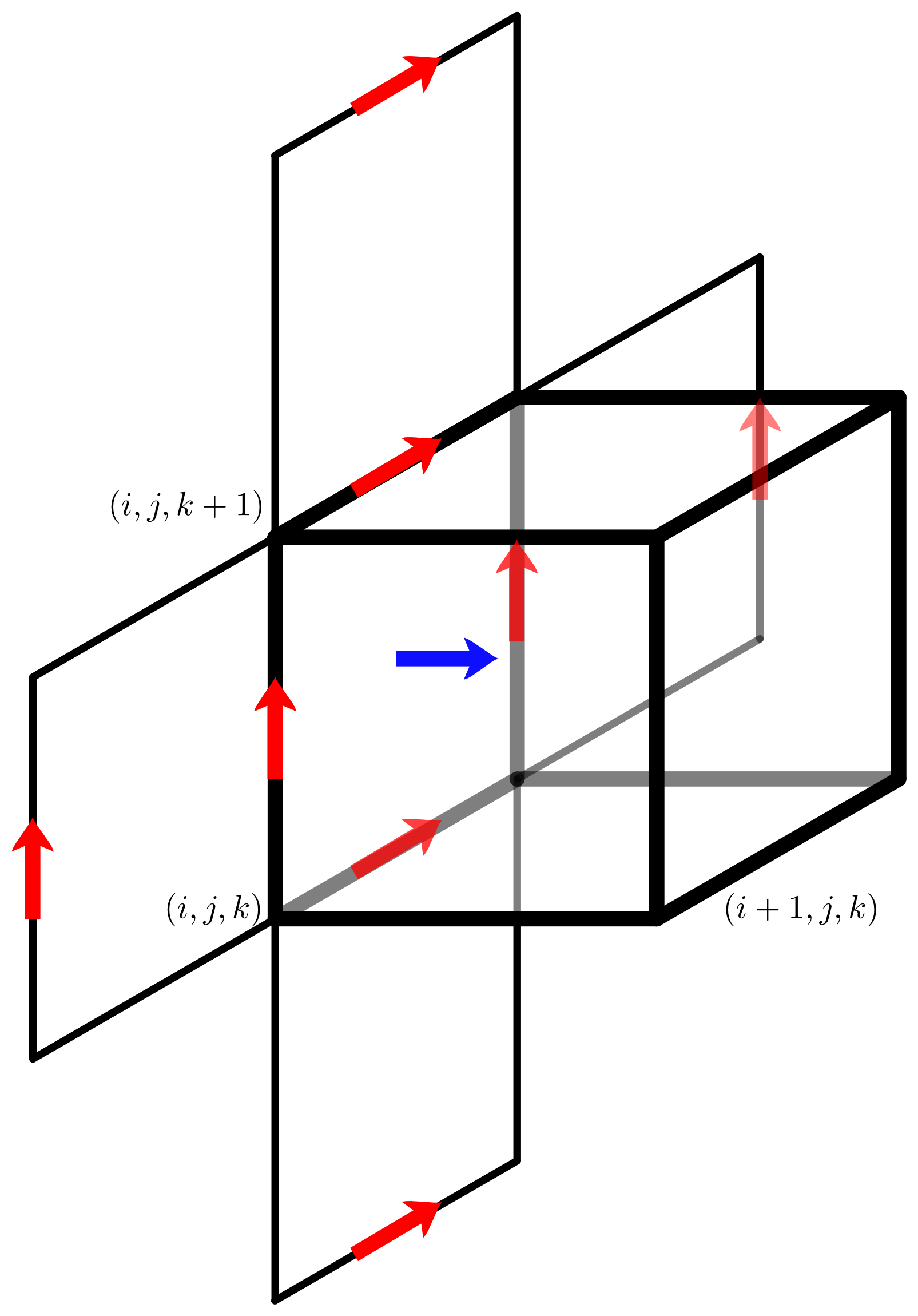
Magnetic Field
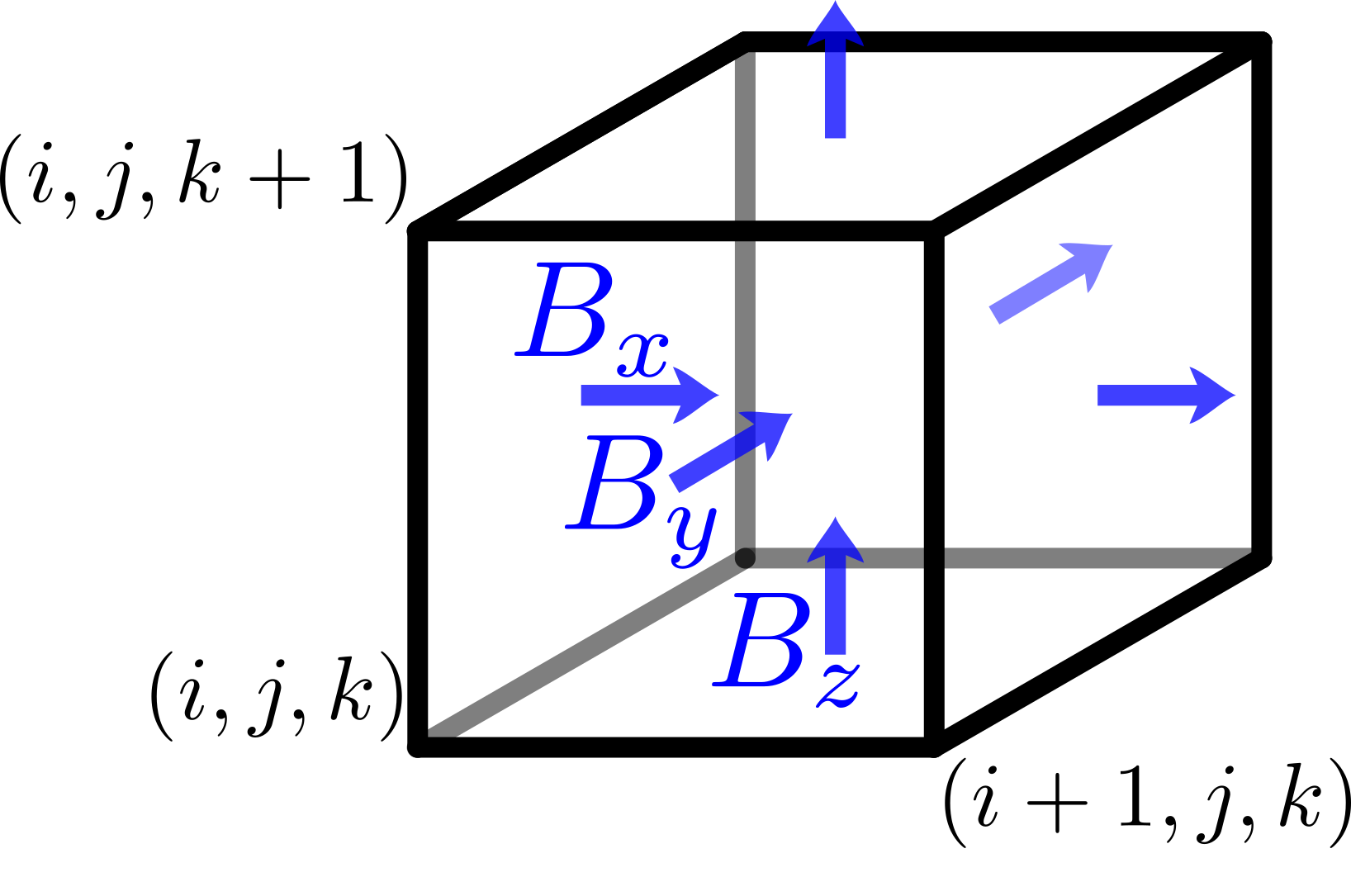
The magnetic field components are located on the dual grid, that is on
the cell faces. The x component B_x of the magnetic field is located
at the center of the face defined by e_y and e_z.
Therefore the electric field components E_y and E_z are located on the
cell edges around the magnetic field component B_x, which is optimal
for the calculation of curl(E)_x that is needed to update B_x.
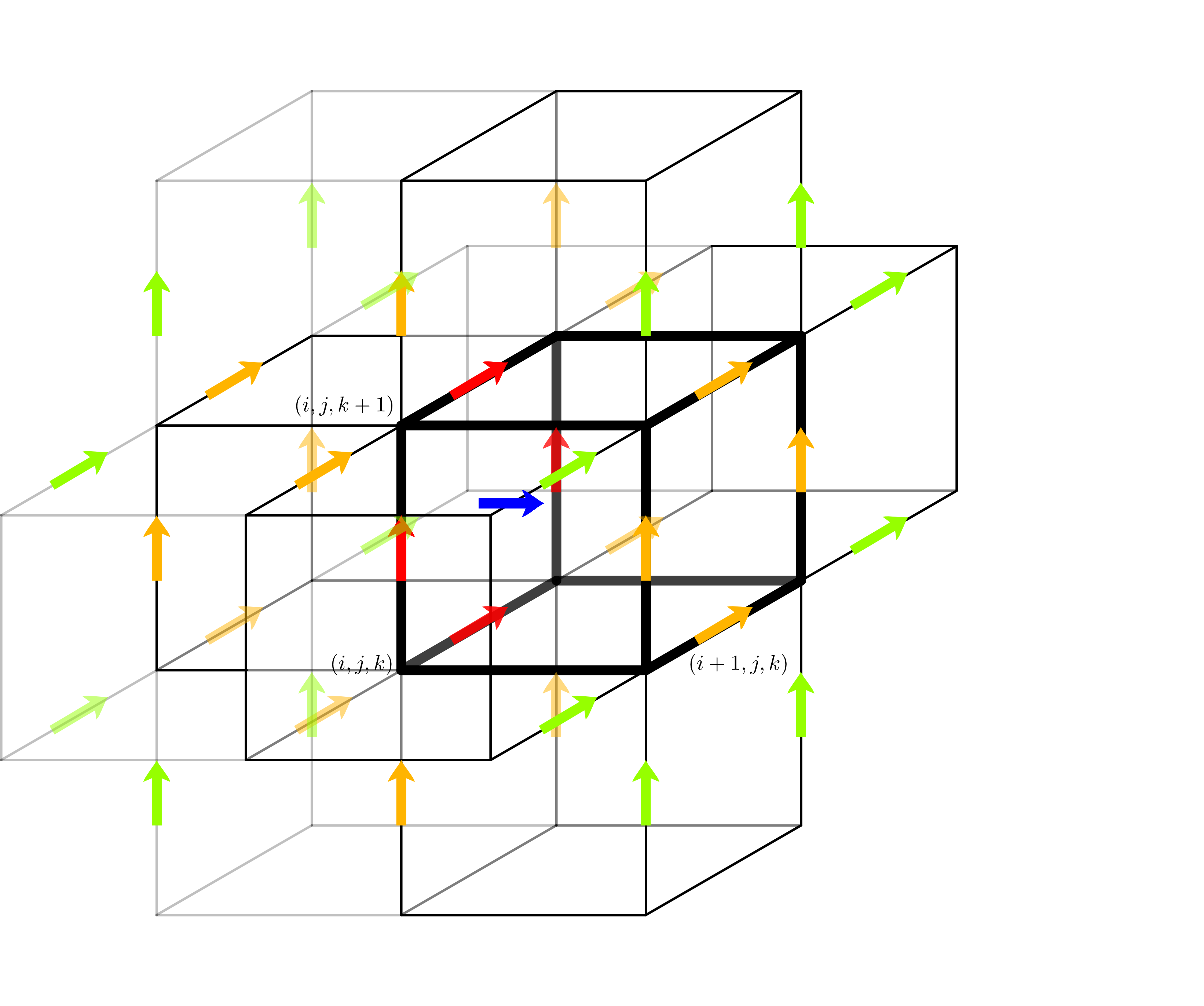
Electric Current
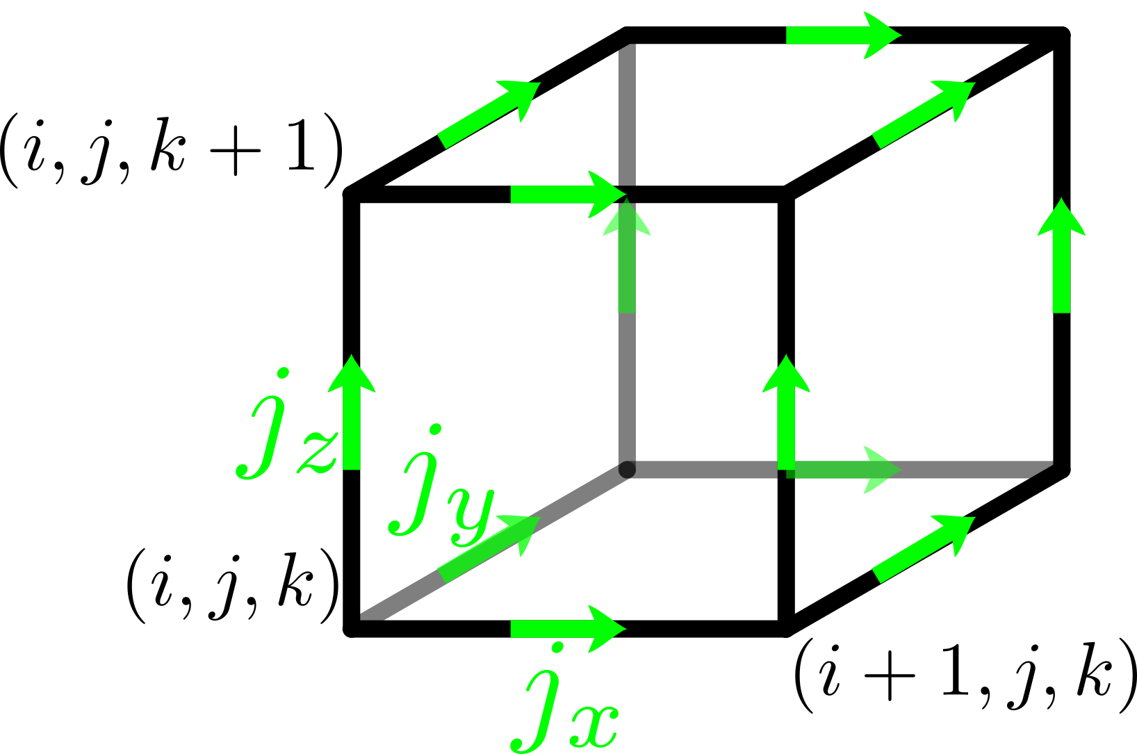
The components of the electric current (and mass flow, if computed for
analysis purposes) are located at the mid points of cell edges.
In the electromagnetic plasma model the update of a component E_i of the
electric field needs the curl curl(B)_i of the magnetic field and the
corresponding component j_i of the current. Therefore it is beneficial
to collocate the current density with the electric field.
Charge Density
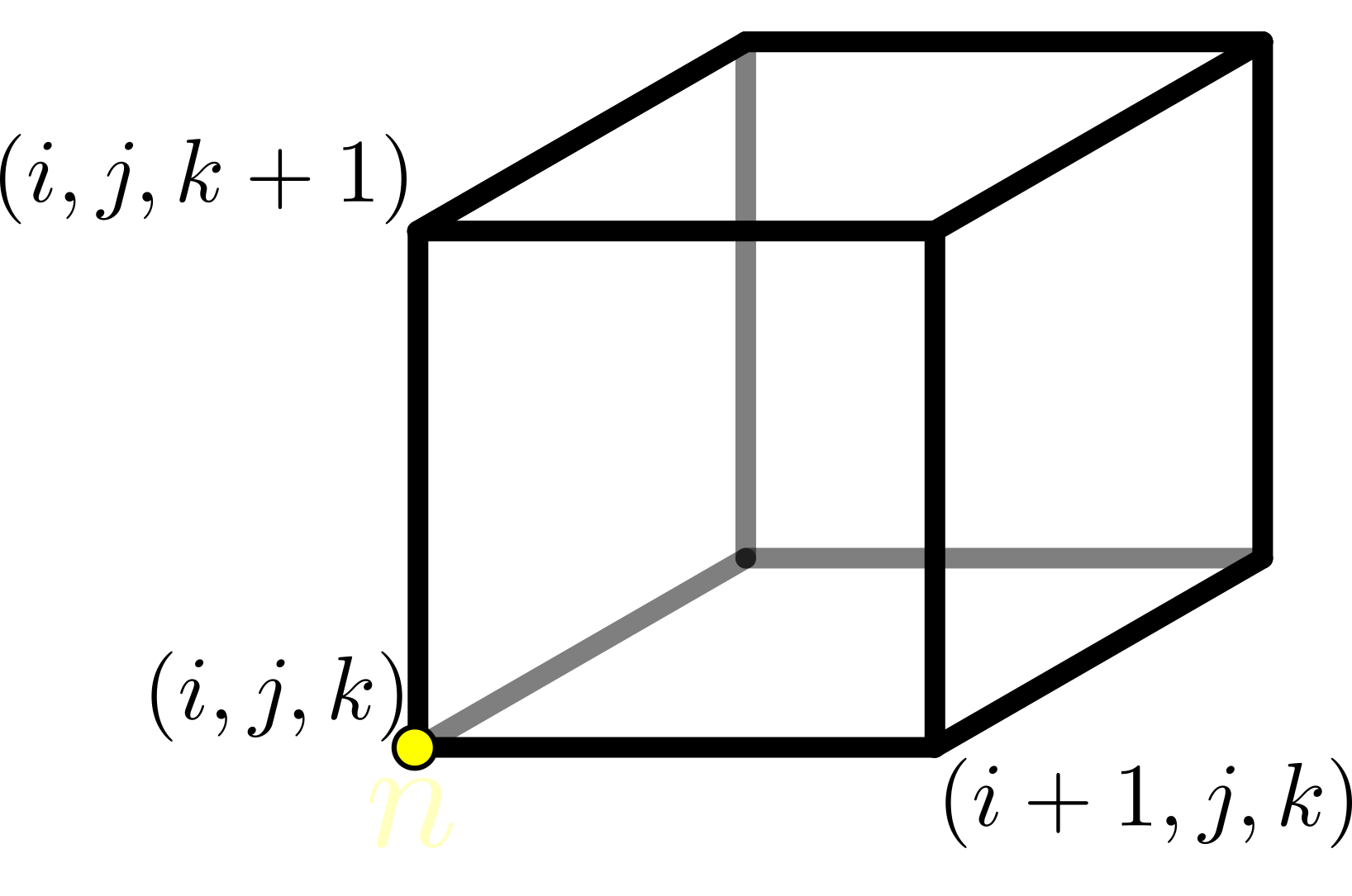
The charge density is located in the corner of the grid cell. The
center of the grid cell would seem more intuitive, as it would then
represent all charges in the cell, but the location in the corner
makes the formulation of the Poisson equation (for the electrostatic
plasma model) and of the discrete continuity equation (when testing the
electromagnetic plasma model) much easier.
Shape Functions
Particle-in-cell codes are, as the name already implies, a mix of an
Eulerian gridded description of the fields and a Langrangian
description of freely moving particles. Connecting the two parts
requires interpolation between the staggered grid described above and
the arbitrary position of a particle. Many different interpolation
schemes have been devised over the years. Schemes that decompose into
products of one-dimensional shape functions can easily be implemented
in ACRONYM and actually a large number of them is supported. The most
commonly used schemes of 1st, 2nd, and 3rd order are shown in a little
bit more detail below. For additional details we refer to the paper
Different Choices of the Form Factor in Particle-in-Cell
Simulations by
Kilian et al., 2013.
Cloud in Cell
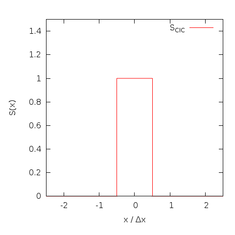
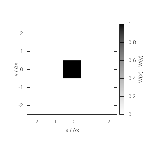
While assigning particles simply to the nearest grid point (NGP) is
possible, this trivial zeroth order interpolation introduces too much
numerical noise to be useful. Assigning a finite size of one grid cell
to particles strongly reduces this noise. The overlap integral between
the charge cloud representing the particle and the grid cell (area
weighting) can be calculated analytically beforehand and the resulting
computation is equivalent to a linear interpolation. This CIC method was
originally introduced by
Birdsall and
Fuss, 1969 and made semi-Langrangian plasma simulations feasible.
Triangular Shaped Cloud
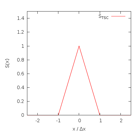
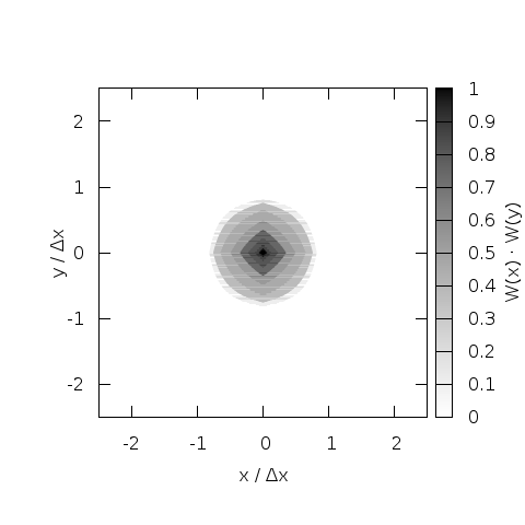
While CIC is a big improvement over NGP, it is not perfect. A widely
discussed (see e.g. chapter 5 in the standard reference
Computer
simulations using particles by Hockney and Eastwood, 1988)
improvement is the triangular shaped cloud (TSC) that replaces the
piecewise defined cloud of CIC with a continuous, piecewise linear
function. This increases the effective size of the particle and the
number of grid cells involved in the interpolation somewhat, but the
reduced noise level and the improved isotropy usually justifies the cost.
Piecewise Quadratic Shape
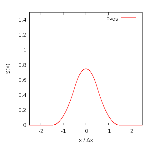
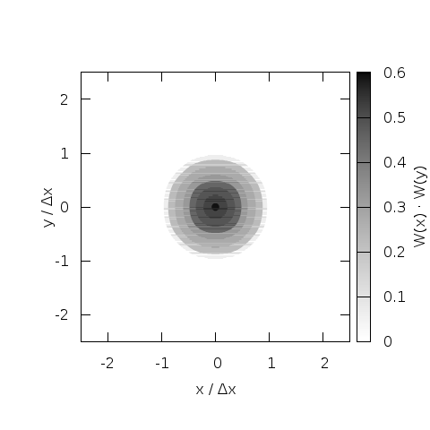
The next higher order interpolation function is the piecewise quadratic
shape (PQS), which is not only continuous, but also differentiable. This
improves roll-off of the Fourier transform by 3dB per octave (a function
that has a discontinuity in the nth derivative has a Fourier transform
that rolls of proportional to 1/k^{n+1}). If the additional cost due to
the growing number of grid cells that are involved in the interpolation
is justified depends on the tolerable noise level and the dimensionality
of the problem.
Current Deposition
Charge deposition is relatively straight forward once a shape function
is selected. For an electrostatic particle-in-cell code it is
sufficient to calculate the electric field and continue. An
electromagnetic code on the other hand needs the electric current as a
source term in the Maxwell solver. Naive deposition (interpolating q*v
at the position of the particle using the shape function directly)
leads to a current distribution that does not satisfy the discrete
continuity equation. This in turn leads to ghost charges, violation of
Gauss law and phantom forces. While it is possible to correct the
computed current distribution to remove these effects (and the code
does support divergence cleaning following the scheme by
Marder, 1987)
it is also possible to construct current deposition schemes that
directly conserve continuity of electric charges.
The code supports two different such schemes (details below).
Additionally it can compute and deposit quantities such as mass density,
mass flow, number density, and moments of the distribution function,
both as a total over all species and separated per species. These
quantities are not needed for the temporal evolution, but can be
valuable diagnostics when investigating the physics of a problem.
Esirkepov
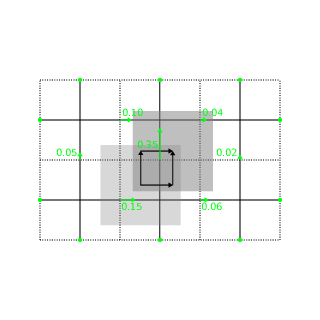
The default current deposition scheme follows the method proposed by
Esirekepov,
2001. It decomposes the particle motion into axis parallel motions
that are weighted in such a way that the correct total current is
produced and charge conservation is satisfied. This method works with
all shape functions and shows good performance.
Umeda
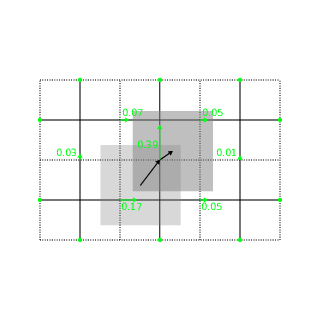
Alternatively the code also supports the current deposition algorithm
by
Umeda,
2003. This algorithm decomposes the particle motion into straight
segments with the constraint that the particle can only cross cell
boundaries at the middle of cell faces. Only CIC and TSC shape
functions are supported. It should be possible to extend this to other
shape functions, but to our knowledge this is beyond the published
state of the art. Main advantage of the deposition method is a
different distribution of numerical noise in k-omega space that might
be advantageous to some simulations.
Field Solver
The ACRONYM code supports a large number of different field solvers,
that have different tradeoff between computational cost, numerical
noise, and accuracy. They can be roughly divided into three classes:
Electrostatic solver, where the electric field is determined by the
charge density through Poissons equation; Electromagnetic solver, where
both electric and magnetic fields are updated self consistently from
the current density; and the radiation free plasma model, which neglects
the displacement current and removes electromagnetic waves by
construction. Warm collisionless plasma (in excess of 1 MK) is usually
best handled by the electromagnetic solvers. However if applicable, the
other solvers can speed up the computations by one or two orders of
magnitude, as the restrictive CFL condition on the time step due to
electromagnetic waves is removed.
Electrostatic
In the electrostatic plasma model the (longitudinal) electric field is
determined by the net charge density of all particles. The Poisson
equation that has to be solved is elliptic, i.e. exhibits instantaneous
propagation and requires a global field solver. While surprising at
first this can be thought of as the limit of long timesteps (much longer
than the propagation time of electromagnetic waves through the
simulation domain) or the limit of infinite speed of light. Transverse
electric fields are not present in this model and the magnetic field is
static. This plasma model is only applicable in the absence of large
electric current and (equivalently) slow (certainly non-relativistic)
particle motion. Depending on the boundary conditions (mixed boundary
conditions are not supported in this plasma model) one of two
different solvers is chosen.
Spectral Solver
If the domain is periodic, the Poisson equation of the electrostatic
plasma model is solved using a spectral solver. The code deposits the
charge density of all particles to the grid and computes the Fourier
transform of it. In Fourier space the Poisson equation can easily be
solved for each different k, allowing for the direct construction of
of the Fourier transform of (one component of) the electric field. A
subsequent inverse Fourier transform produces the electric field in
real space. The global Fourier transform over all spatial dimensions
is computed using a modified version of the
Sandia
FFT that allows to use
FFTW 3 as
the underlying local 1d transformation. Two features that are described
in the literature but not used in all codes are the direct computation
of the electric field instead of the potential, which requires two
additional inverse Fourier transformations but provides slightly more
accurate fields, and the use of the so-called sinc softening.
Solver using Greens Functions
If open / absorbing boundaries are desired in the electrostatic model,
a different solver is used. It also uses the charge density, but then
convolves that with the Greens function of free space to determine the
electric field. The convolution is performed in Fourier space, where it
is a simple point by point multiplication. The Fourier transformed of
the charge density is determined directly from the charge density in
each time step. The Fourier transformed of the Greens function is
determined once, at startup by evaluation of an analytic expression for
the Greens function on a double sized (to avoid wraparound in Fourier
space) grid followed by a Fourier transformation. After the convolution
/ multiplication in Fourier space an inverse Fourier transform is
necessary for each field component to determine the electric field in
real space.
Electromagnetic
The most widely used plasma model in ACRONYM is the electromagnetic
plasma model where both electric and magnetic fields are updated
selfconsistently. In the initial setup the electric field is usually
set to zero and the magnetic field is set to some (divergence-free!)
profile determined by the specific setup. In each timestep the electric
field is updated based on the curl of the magnetic field and the
electric current, before the magnetic field is leap-frogged over it
using the curl of the new electric field. (Actually the magnetic field
update is split into two half-steps to have the electric and magnetic
fields available at the same instant in time to update the particles.)
While the details of the calculation of the current density that enters
as a source term is shifted to the current deposition, the numerical
approximation of the curl is retained directly in the electromagnetic
field solver. Different finite differences approximations are
implemented in the code:
Yee
The code of course implements the standard algorithm by
Yee, 1966 that
also drives the grid layout for the field quantities.
In this algorithm the curl of the electric field that is necessary to
update B_x is computed from the four components of E_y and E_z that
surround B_x in the staggered grid. The algorithm is straight forward
and guarantees that the magnetic field does not gain a non-physcial
divergence.
This algorithm is 2nd order accurate in dx, but is somewhat anisotropic
and exhibits significant numerical dispersion along the coordinate axes.
4th Order
In an attempt to improve the field solver a (naive) solver that is
4th order accurate was implemented. This solver uses additional grid
location of E_y and E_z to compute curl(E) that enters the update of
B_x. The big advantage is that it requires very limited modification
of the code as the same grid layout can be used. The major downside is
that the higher order of convergence is not visible at typical cell
spacings and that smaller cell spacings where the faster convergence
would be beneficial are typically prohibitively expensive.
NSFD (CK, CK5)
The big improvement came with the realization that order of convergence
is not as important as the error constant in front of the leading term.
Here the
non
standard
finite
differences
schemes proposed by
Cole,
1997 and
K�rkk�inen,
2006 excel. They use additional grid locations to compute the curl
and optimize their relative weights to obtain numerical approximations
of the curl operator that combine 2nd order accuracy with other
desirable properties. A paper by
Vay et al., 2011
discusses a number of potential parameters of such NSFD schemes.
ACRONYM implements (in the nomenclature used there) the schemes CK and
CK5, that offer maximally long time steps and maximally isotropic
propagation, respectively.
M24
In another modification of the Yee scheme
Hadi, 1997 has proposed
to use the grid locations used by the Yee scheme, the naive 4th
order solvers and the grid location required to close the big outer
loop. Again different relative weights are possible.
Greenwood et al.,
2004 have shown that a carefully chosen set of parameters can
change the phase speed of electromagnetic waves suitably to remove grid
Chernenkov effects. The scheme is not perfect and can therefore not
remove grid Chernenkov radiation under all conditions, but the common
case of axis parallel beams profits significantly. If Chernenkov
radiation is still an issue the solver can be combined with
Friedman
filtering.
Radiation Free (Darwin)
While the electrostatic plasma model neglects all effects O(v/c) and
the electromagnetic model retains the finite speed of light, it is also
possible to construct a plasma model that retains effects up to
O(v^2/c^2), but ignores higher order effects. Interestingly enough there
is a unique construction that does that which is equivalent to removing
the displacement current and thus removing electromagnetic radiation.
This results in longitudinal fields identical to the electrostatic
plasma model, some transverse electric fields (but no light waves), and
some corrections to the background magnetic field. Unfortunately the
solver is quite complex and follows some unpublished work by Decyk. The
biggest challenge is that the equation for the transverse electric
field E_T needs the temporal change of the current density d j/dt as an
input. Calculating this quantity from standard current deposition is
too noisy. It is possible to rewrite the term, but at the cost of
extra, numerically expensive, deposition steps.
Boundary Conditions
The code in general allows for several boundary conditions, that can
be different for different ends of the simulation domain. (Of course a
periodic boundary at the lower end of the x axis needs to be connected
to a periodic boundary at the upper end of the same axis.) The main
challenge when creating boundary conditions is the need to have full
consistency between the boundary formulation for the electromagnetic
fields and the boundary conditions for the particles. Discrepancies lead
to the formation of charged layers in the best case and violent
instabilities in the worst case. Periodic boundary conditions are the
easiest and most widely supported boundary conditions. Reflective
boundary conditions are only supported by the electromagnetic plasma
model. Absorbing boundary conditions are at least supported by
electrostatic and electromagnetic solvers.
Periodic Boundary Conditions
Periodic boundary conditions are straight forward and are actually
handled internally in the same way as the interior inter-task
boundaries, i.e. particles are sent to the new CPU and field values are
copied into ghost zones. The wrap around is handled transparently by
the geometry of the MPI Cartcom.
Perfect Electric Conductor
Metal walls with perfect electric conductivity are modeled by setting
the tangential electric field to zero. The current densities of
particles close to the metal wall are adjusted using the current of an
imaginary mirror charge on the other side of the wall. Since these
boundary conditions are reflective to electromagnetic waves they are
complemented on the particle side with specular reflection of incident
particles. Unlike a real metal wall no charged particles are absorbed
or reflected.
Absorbing Boundary Conditions
The absorbing boundary conditions are implemented using a perfectly
matched layer. Many different PML formulations exist. The current
implementation uses an unsplit formulation. To improve absorption of low
frequency waves a complex frequency shift approach is used, that
requires a convolutional PML, i.e. the storage of auxiliary fields in
the boundary region. On the particle side, outgoing particles are
simply removed. The injection of new particles is handled by filling
the ghost zone with new particles, performing one timestep inside the
ghost zone and keeping the particles that enter the simulation domain.
Output
Field quantities are written to self-describing HDF5 files in Pixie
format using parallel HDF5 (i.e. one HDF5 file per simulation, for all
CPUs and all timesteps). Particle data can be written to HDF5 tables
or to binary files using MPI-IO.
